Comparing Different Query Strategies
Example file: examples/plot.py
This example shows the basic way to compare two active learning algorithm. The
script is located in /examples/plot.py. Before running the script, you
need to download sample dataset by running /examples/get_dataset.py and
choose the one you want in variable dataset_filepath.
1 | # Specifiy the parameters here:
|
First, the data are splitted into training and testing set:
1 2 3 4 5 6 7 8 9 10 11 | def split_train_test(dataset_filepath, test_size, n_labeled):
X, y = import_libsvm_sparse(dataset_filepath).format_sklearn()
X_train, X_test, y_train, y_test = \
train_test_split(X, y, test_size=test_size)
trn_ds = Dataset(X_train, np.concatenate(
[y_train[:n_labeled], [None] * (len(y_train) - n_labeled)]))
tst_ds = Dataset(X_test, y_test)
fully_labeled_trn_ds = Dataset(X_train, y_train)
return trn_ds, tst_ds, y_train, fully_labeled_trn_ds
|
The main part that uses libact is in the run function:
1 2 3 4 5 6 7 8 9 10 11 12 13 14 15 | def run(trn_ds, tst_ds, lbr, model, qs, quota):
E_in, E_out = [], []
for _ in range(quota):
# Standard usage of libact objects
ask_id = qs.make_query()
X, _ = zip(*trn_ds.data)
lb = lbr.label(X[ask_id])
trn_ds.update(ask_id, lb)
model.train(trn_ds)
E_in = np.append(E_in, 1 - model.score(trn_ds))
E_out = np.append(E_out, 1 - model.score(tst_ds))
return E_in, E_out
|
In the for loop on line 25, it iterates through each
query in active learning process. qs.make_query returns the
index of the sample that the active learning algorithm wants to query.
lbr acts as the oracle and lbr.label returns the
label of the given sample answered by oracle. ds.update updates
the unlabeled sample with queried label.
A common way of evaluating the performance of active learning algorithm is to
plot the learning curve. Where the X-axis is the number samples of queried, and
the Y-axis is the corresponding error rate. List E_in,
E_out collects the in-sample and out-sample error rate after each
query. These information will be used to plot the learning curve. Learning curve
are plotted by the following code:
1 2 3 4 5 6 7 8 9 10 11 | # Plot the learning curve of UncertaintySampling to RandomSampling
# The x-axis is the number of queries, and the y-axis is the corresponding
# error rate.
query_num = np.arange(1, quota + 1)
plt.plot(query_num, E_in_1, 'b', label='qs Ein')
plt.plot(query_num, E_in_2, 'r', label='random Ein')
plt.plot(query_num, E_out_1, 'g', label='qs Eout')
plt.plot(query_num, E_out_2, 'k', label='random Eout')
plt.xlabel('Number of Queries')
plt.ylabel('Error')
plt.title('Experiment Result')
|
The following figure are the result of using the diabetes dataset with
train_test_split and LogisticRegression’s
random_state set as 0, and random.seed(0). The E_out line are
removed for simplicity.
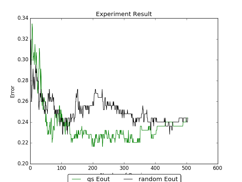
We can see from the example that uncertainty sample is able to reach lower error rate faster than random sampling.
Full source code:
1 2 3 4 5 6 7 8 9 10 11 12 13 14 15 16 17 18 19 20 21 22 23 24 25 26 27 28 29 30 31 32 33 34 35 36 37 38 39 40 41 42 43 44 45 46 47 48 49 50 51 52 53 54 55 56 57 58 59 60 61 62 63 64 65 66 67 68 69 70 71 72 73 74 75 76 77 78 79 80 81 82 83 84 85 86 87 88 89 90 91 92 93 94 95 96 97 98 99 | #!/usr/bin/env python3
"""
The script helps guide the users to quickly understand how to use
libact by going through a simple active learning task with clear
descriptions.
"""
import copy
import os
import numpy as np
import matplotlib.pyplot as plt
try:
from sklearn.model_selection import train_test_split
except ImportError:
from sklearn.cross_validation import train_test_split
# libact classes
from libact.base.dataset import Dataset, import_libsvm_sparse
from libact.models import *
from libact.query_strategies import *
from libact.labelers import IdealLabeler
def run(trn_ds, tst_ds, lbr, model, qs, quota):
E_in, E_out = [], []
for _ in range(quota):
# Standard usage of libact objects
ask_id = qs.make_query()
X, _ = zip(*trn_ds.data)
lb = lbr.label(X[ask_id])
trn_ds.update(ask_id, lb)
model.train(trn_ds)
E_in = np.append(E_in, 1 - model.score(trn_ds))
E_out = np.append(E_out, 1 - model.score(tst_ds))
return E_in, E_out
def split_train_test(dataset_filepath, test_size, n_labeled):
    X, y = import_libsvm_sparse(dataset_filepath).format_sklearn()

    X_train, X_test, y_train, y_test = \
        train_test_split(X, y, test_size=test_size)
    trn_ds = Dataset(X_train, np.concatenate(
        [y_train[:n_labeled], [None] * (len(y_train) - n_labeled)]))
    tst_ds = Dataset(X_test, y_test)
    fully_labeled_trn_ds = Dataset(X_train, y_train)

    return trn_ds, tst_ds, y_train, fully_labeled_trn_ds
def main():
# Specifiy the parameters here:
# path to your binary classification dataset
dataset_filepath = os.path.join(
os.path.dirname(os.path.realpath(__file__)), 'diabetes.txt')
test_size = 0.33 # the percentage of samples in the dataset that will be
# randomly selected and assigned to the test set
n_labeled = 10 # number of samples that are initially labeled
# Load dataset
trn_ds, tst_ds, y_train, fully_labeled_trn_ds = \
split_train_test(dataset_filepath, test_size, n_labeled)
trn_ds2 = copy.deepcopy(trn_ds)
lbr = IdealLabeler(fully_labeled_trn_ds)
quota = len(y_train) - n_labeled # number of samples to query
# Comparing UncertaintySampling strategy with RandomSampling.
# model is the base learner, e.g. LogisticRegression, SVM ... etc.
qs = UncertaintySampling(trn_ds, method='lc', model=LogisticRegression())
model = LogisticRegression()
E_in_1, E_out_1 = run(trn_ds, tst_ds, lbr, model, qs, quota)
qs2 = RandomSampling(trn_ds2)
model = LogisticRegression()
E_in_2, E_out_2 = run(trn_ds2, tst_ds, lbr, model, qs2, quota)
    # Plot the learning curve of UncertaintySampling to RandomSampling
    # The x-axis is the number of queries, and the y-axis is the corresponding
    # error rate.
    query_num = np.arange(1, quota + 1)
    plt.plot(query_num, E_in_1, 'b', label='qs Ein')
    plt.plot(query_num, E_in_2, 'r', label='random Ein')
    plt.plot(query_num, E_out_1, 'g', label='qs Eout')
    plt.plot(query_num, E_out_2, 'k', label='random Eout')
    plt.xlabel('Number of Queries')
    plt.ylabel('Error')
    plt.title('Experiment Result')
plt.legend(loc='upper center', bbox_to_anchor=(0.5, -0.05),
fancybox=True, shadow=True, ncol=5)
plt.show()
if __name__ == '__main__':
main()
|